Double descent is when test error falls, peaks at the interpolation threshold, then falls again as models grow. Why it happens, and whether it is real.

Updated October 2026
Double descent is a pattern in machine learning where a model's test error falls, rises to a peak, and then falls again as the model gets larger. The peak sits at the interpolation threshold, the size at which the model can just fit every training example exactly. Past that threshold, adding parameters lowers test error again, often below the best unregularized smaller model.
That second fall contradicts a rule of thumb most statistics courses teach: a model too complex for its data overfits and gets worse. Belkin and colleagues named the pattern in 2019. They argued it reconciles classical theory with modern practice, where networks with far more parameters than training examples still predict well.
Double descent describes test error as a function of model complexity, usually counted as the number of parameters. The curve has two regimes separated by one threshold. In the under-parameterized regime, the model is too small to fit every training example exactly, and test error follows the familiar U shape. At the interpolation threshold, the model can just fit the training data exactly, and test error peaks. In the over-parameterized regime, many exact fits exist, the training procedure picks one of them, and test error falls again. In linear models the threshold sits where parameters equal training examples. In deep networks it depends on the architecture and the training procedure, not on a parameter count alone.
Model size is not the only axis the curve appears on. The same rise and fall can unfold over training time, and a related effect appears as the training set grows, which gives double descent its three types.
Despite the name, double descent is not a form of gradient descent. "Descent" here describes the shape of the error curve, not an optimization method.
The phases show up clearly in a small experiment. A random-features regression model learns a noisy linear function of 10 inputs from 50 training points, with label noise of standard deviation 0.5. The model's size is its number of random ReLU features, each a fixed random direction in the input followed by a cutoff at zero. Only the weights on those features are fit, by least squares, and when many fits are exact the method returns the one with the smallest weights. Test error is the mean squared error against the noiseless function on 2,000 new points. Each of 40 random draws resamples the data, the noise, and the features, and the figures below are medians across draws.
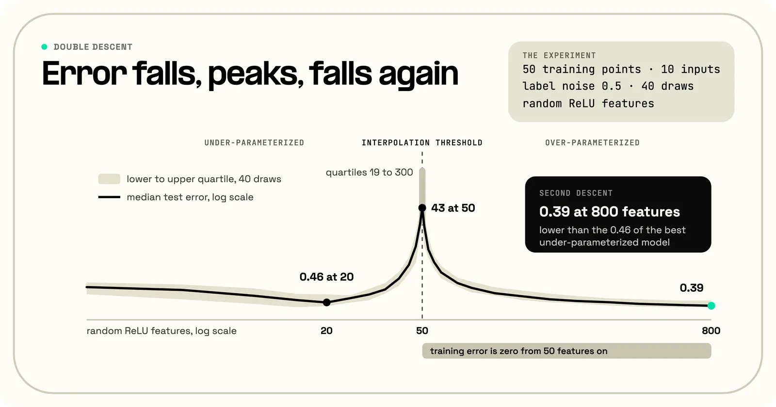
With few features, the model underfits, and test error falls as features are added. It bottoms out at 20 features, at 0.46. Beyond that, the model starts fitting the noise in its 50 training labels, and test error climbs. Up to this point the curve is the classical U.
At exactly 50 features, the model has one weight per training point and can fit all 50 exactly, so training error drops to zero. There is then only one way to fit them, and median test error reaches 43, more than 90 times the best small model. The spread across draws is huge, from 19 to 300 between the lower and upper quartiles. The height of the peak depends on how close the feature matrix comes to being singular in each draw.
Past 50 features, many different fits pass through all the training points, and test error falls steadily as features are added. At 800 features, median test error is 0.39, lower than the 0.46 of the best under-parameterized model, though 800 features beat 20 in only 23 of the 40 draws.
Double descent happens because the model's fit at the threshold is forced, and its fit far past the threshold is chosen. At the threshold, exactly one set of weights fits the training data. Finding it means inverting a feature matrix that is close to singular, so some directions get divided by tiny numbers, and any noise in those directions is amplified into very large weights. In the example, the median length of the weight vector, with every feature on the same scale, jumps from 2.3 at 20 features to 32 at 50. Large weights make predictions swing between the training points, which is variance, and variance peaks at the threshold.
Past the threshold, the training procedure has a choice among many exact fits, and least squares with the smallest-weight rule spreads the fit across more features, so each weight shrinks. By 800 features the median length is down to 0.68. Gradient descent started from zero converges to the same smallest-weight fit in linear models, which is one way the training procedure, and not only the architecture, decides where a model lands. Hastie, Montanari, Rosset, and Tibshirani derived precise formulas for the test error of this fit in linear regression, including the peak where parameters equal samples. In their analysis, error always comes down from the peak, but whether it falls below the best under-parameterized error is conditional. In the simplest case, with independent features that capture the whole signal, it does not. The over-parameterized side can win when the features miss part of the signal and the signal outweighs the noise. Both hold in the example: ReLU features cannot represent a linear target exactly, and the signal's variance is about four times the noise's.
What the features cannot explain sets the height of the peak, together with how close to singular the feature matrix is. Label noise is the obvious part of it, but not the only one. With the noise set to zero, the same experiment still peaks at 50 features, at a median error of 7.2 against 0.30 at 20. It then falls to 0.007 at 800. The forced fit amplifies the part of the target the features miss. For deep networks the same story is an intuition rather than a proof. Nakkiran and colleagues describe a network just able to fit its data as forced to wreck its overall structure to fit noisy or mis-specified labels. A much larger network trained with stochastic gradient descent can absorb that noise and still generalize. They note the argument is proven for linear models and open for neural networks.
Double descent is real in the sense that it reproduces across model families, datasets, and research groups. Whether it matters for a given model depends on regularization and on how complexity is counted.
The evidence starts with Belkin and colleagues, who showed the curve for random Fourier features, two-layer fully connected neural networks, and boosted decision trees and random forests. Nakkiran and colleagues then measured it in convolutional networks, ResNets, and transformers. Their image-classification peaks were strongest with label noise added. On clean labels the peak often flattened into a plateau, and many of the effects disappeared when the authors kept the checkpoint with the lowest test error. Clean-label ResNets on CIFAR-100 were an exception on both counts.
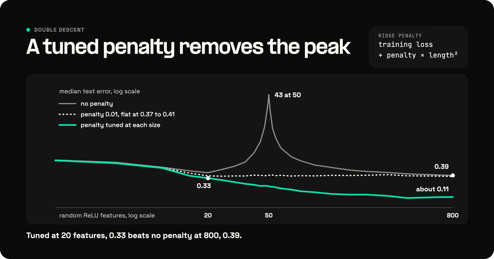
The first caveat is regularization. Nakkiran, Venkat, Kakade, and Ma proved that optimally tuned ridge regularization removes the peak in certain linear regression settings, and showed that it can mitigate the peak in more general models, including neural networks. A ridge penalty adds a multiple of the squared weight length to the training loss, and the computed example bears out their result. With a penalty of 0.01, the peak disappears: median error stays between 0.37 and 0.41 from 20 features to 800, and is 0.40 at 50. With the penalty retuned separately at each size, error falls as features are added: 0.33 at 20, 0.21 at 50, and about 0.11 from 400 features on. The tuned penalty here is the best of 10 values by test error; a real project would choose it on a validation set.
Those numbers cut both ways, at least in this example. A tuned 20-feature model, at 0.33, beats the unregularized 800-feature model, at 0.39, so here tuning the penalty buys more than the unregularized second descent does. Size still pays once the penalty is retuned at each size: the tuned 800-feature model beats the tuned 20-feature one by a factor of three. With the penalty fixed at 0.01, it does not, because that curve is flat from 20 features to 800.
The second caveat is counting. Curth, Jeffares, and van der Schaar argued that in trees, boosting, and linear regression, the parameter count grows along two axes, one after the other. Random forests are the clearest case. Belkin's forest curve first grows one tree until it can fit every training point, then adds more trees to the ensemble. The second descent begins exactly where the curve switches from the first axis to the second. Measured with an effective parameter count, a measure of how much flexibility the fitted model actually uses when it predicts new points, those curves fold back into the usual U. The measure counts on new points rather than training points and tracks variance, so it can exceed a model's raw parameter count: a 30-feature fit scores about 87. Applied to the computed example, it puts the 800-feature fit at about 88 effective parameters, not 800, and shows the count falling steadily past the threshold. It does not fold this curve into a single U, though. At the same effective count, the 30-feature fit has a median error of 0.67 against 0.39 at 800 features. The variance part is the same for both, so the gap is bias: 0.22 for the 30-feature fit, 0.007 for the 800-feature fit.
So double descent is neither a myth nor a law. The peak is what unregularized models do at the interpolation threshold. A tuned penalty removes it in certain linear models and in the computed example, and shrinks it in the networks tested. Size past the threshold still pays in the example, once the penalty is retuned at each size. A better measure of complexity explains part of the curve and, in some experiments, turns it back into a U. The lesson that survives every caveat is that raw parameter count is a poor guide to how much a model overfits.
Double descent extends the bias-variance trade-off rather than overturning it. The trade-off splits test error into bias, which falls as a model gains flexibility, and variance, which rises, and it predicts the U-shaped curve of the under-parameterized regime correctly. What breaks past the interpolation threshold is the use of parameter count as the measure of flexibility: variance falls again because the training procedure picks smaller-weight fits, even as the parameter count grows. In the computed example, both parts spike at the threshold, variance far more than bias: 143 against 7.2 at 50 features. Both fall past it, and bias ends at 0.007 at 800 features against 0.30 at 20. That is the counting caveat seen from the classical side. The classical curve is the left half of the double descent curve, drawn with a complexity measure that stops working at the threshold.
The three types of double descent differ in what increases along the horizontal axis. Model-wise double descent is the classic version, with test error plotted against model size. Epoch-wise double descent appears when a large network trains for longer. Training raises how much data the network can fit, so a long run carries it through the point where it just fits its training set, and test error falls, rises, and falls again. Sample-wise non-monotonicity is the counterintuitive one. Adding training data raises the size a model needs to fit it, which moves the peak toward larger models, so a fixed model near the peak can get worse with more data. Nakkiran and colleagues measured all three in neural networks.
The classical view of model complexity comes from the bias-variance analysis that Geman, Bienenstock, and Doursat applied to neural networks in 1992, which made the U-shaped curve the standard picture. Curves with a second descent appeared in scattered work on simple classifiers and linear regression from 1989 onward, as Loog and colleagues later documented, but they were treated as oddities. Belkin and colleagues named the pattern in 2019 and connected it to the success of over-parameterized networks. Nakkiran and colleagues extended it to deep learning the same year, and the 2023 work of Curth and colleagues reopened the question of how much of it depends on how complexity is measured.
Double descent is not the same as grokking, although both involve a model generalizing after it has already fit its training data. Double descent is a curve of test error against model size, training time, or data. Grokking, described by Power and colleagues in 2022, is a sudden jump in test accuracy long after training accuracy reaches 100%, seen on small algorithmic tasks such as modular arithmetic. Epoch-wise double descent and grokking are the closest pair, since both unfold over training time.
Double descent means that test error descends twice as a model grows: once in the usual under-parameterized regime, and again after a peak at the size where the model can first fit its training data exactly. The name describes the shape of the curve.
Double descent happens because a model just large enough to fit its training data has only one way to do it. Finding that fit amplifies label noise, and any part of the target the model cannot represent, into very large weights. A much larger model has many exact fits to choose from, and training procedures such as gradient descent tend to pick small-weight fits that generalize better. The account is proven for linear models and an intuition for deep networks.
Mikhail Belkin, Daniel Hsu, Siyuan Ma, and Soumik Mandal named double descent in a 2019 paper in the Proceedings of the National Academy of Sciences. Curves with the same shape had appeared earlier, in work on simple classifiers and linear regression going back to 1989, and Preetum Nakkiran and colleagues extended the idea to deep learning in 2019.
Double descent is not a type of gradient descent; "descent" names the shape of the error curve. The two are connected in one way: gradient descent's preference for small-weight solutions is part of why test error falls again past the interpolation threshold.
This content was generated with the assistance of AI. Our AI prompt chain workflow is carefully grounded and preferences .gov and .edu citations when available. All content is reviewed by a Telnyx employee to ensure accuracy, relevance, and a high standard of quality.