What are diffusion models? How they work, types, and examples

Updated October 2026

A diffusion model is a generative AI model that creates new data, most often images, by starting from random noise and removing it step by step. The model learns this from the opposite process: real training examples are buried in noise a little at a time, and the model is trained to predict the noise added at each step. Generation repeats that prediction, starting from pure noise, until a new sample remains.

In its standard form, a diffusion model is trained on one task: predicting the noise in a noisy input. In Ho, Jain and Abbeel's 2020 paper, one image took 1,000 of those predictions.

The same loop generates images in Stable Diffusion and DALL-E 2, video in OpenAI's Sora, and speech in several text-to-speech systems.

What is a diffusion model?

A diffusion model is a generative AI model that makes data by learning to undo a gradual noising process.

Generative adversarial networks, variational autoencoders and the autoregressive transformers behind large language models are the other main types.

Diffusion models get their name from physics. Sohl-Dickstein and colleagues introduced the method in 2015, borrowing from non-equilibrium thermodynamics.

Their forward process spreads the data's structure out until none is left, the way a drop of ink diffuses through water.

In psychology, the same name belongs to the drift-diffusion model of two-choice decisions, an unrelated idea. This page covers the generative AI sense.

How do diffusion models work?

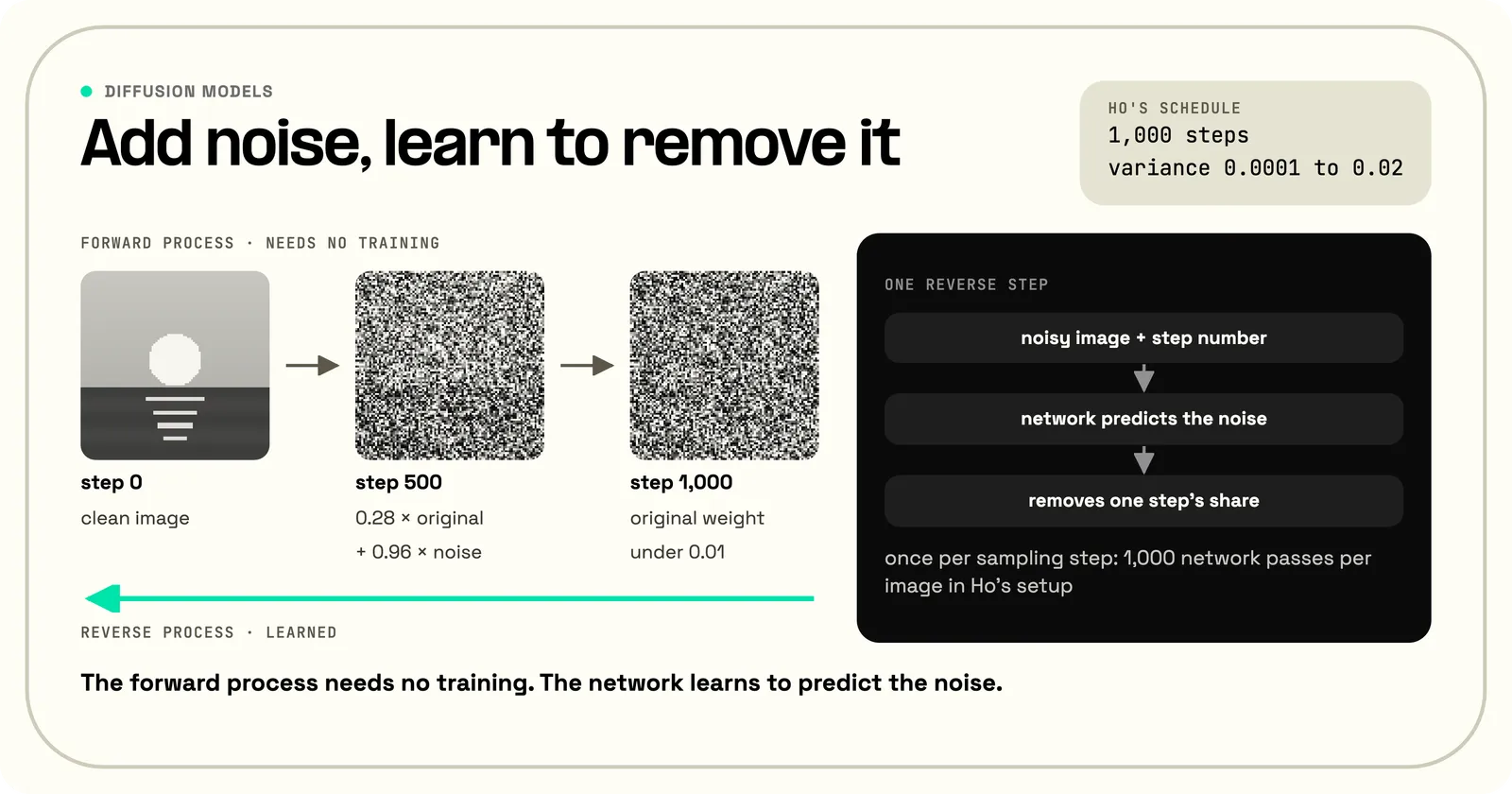
A diffusion model works through two processes: a fixed forward process that adds noise to data until nothing recognizable is left, and a learned reverse process that removes it.

The forward process needs no training. At each step it shrinks the sample slightly and adds a little Gaussian noise, the bell-curve random noise of statistics. Each step depends only on the one before, so the process is a Markov chain.

Ho and colleagues used 1,000 steps. The noise variance added per step rose linearly from 0.0001 to 0.02, and each step scaled the sample by the square root of 1 minus that variance.

Those small steps compound. The original's weight at any step is the square root of the product of (1 minus the variance) over every step so far, and the noise weight is the square root of 1 minus that product.

At step 500 the noisy image is 0.28 times the original plus 0.96 times fresh noise. By step 1,000 the original's weight is under 0.01.

Because that formula needs only the clean image, the noisy version at any step can be computed in one jump.

Training the reverse process, a neural network, uses that shortcut. Training picks a real image and a random step, noises the image to that step in one jump, and asks the network to predict the noise that was added.

The loss is the squared difference between the true noise and the network's guess. It simplifies the full objective, a sum of KL divergence terms. Ho and colleagues found the simpler loss gave better images.

Generation runs the network once per sampling step. The model starts from pure noise, predicts the noise in it, and removes one step's share of that prediction, which lands it at the next noise level down.

A DDPM, the original form, uses one sampling step per noise level: 1,000 network passes per image in Ho's setup. It also adds a little fresh random noise back at each step, which makes each run random.

What architecture do diffusion models use?

A diffusion model's denoiser is a neural network with three inputs, the noisy sample, the step number and any condition such as a text prompt, and one output: its estimate of the noise.

Image models first used a U-Net, a convolutional network that shrinks an image to a compact representation and expands it back, with shortcuts between layers of matching size.

Newer image and video models use a transformer as the denoiser. Peebles and Xie replaced the U-Net with a diffusion transformer that treats patches of a compressed image as tokens. Image quality improved steadily as they made it larger.

OpenAI describes Sora as a diffusion transformer too. The transformer is the network inside; diffusion is how that network generates. "Diffusion model or transformer" is not an either-or choice.

How do diffusion models generate images from text?

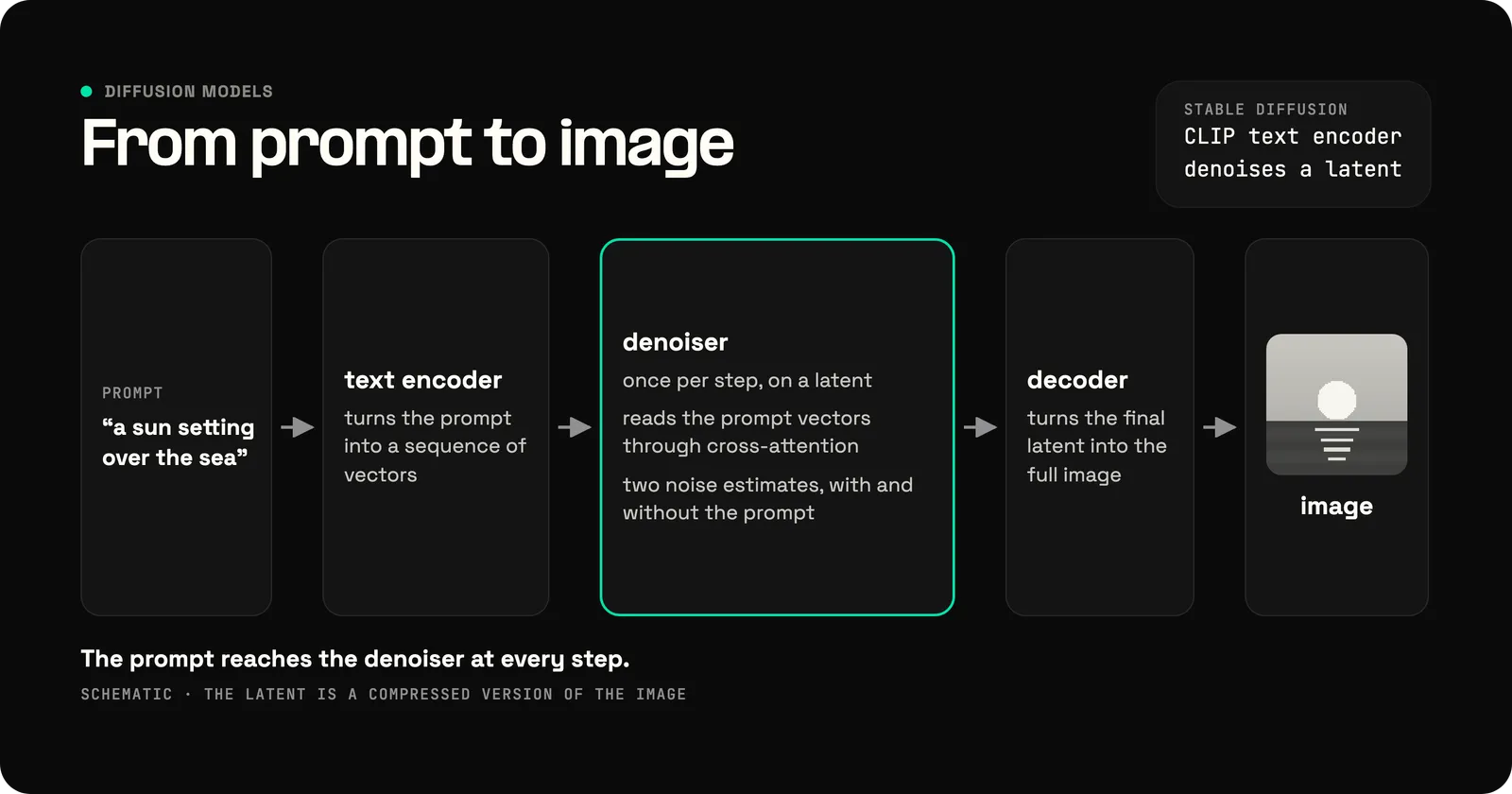
A text-to-image diffusion model feeds an encoded version of the prompt to the denoiser at every step, so each noise estimate is pulled toward images that match the words.

A separate text encoder turns the prompt into a sequence of vectors first. Stable Diffusion uses the text encoder from CLIP, a model trained to match images with their captions. Imagen uses T5, a text-only language model.

The denoiser reads the prompt vectors through cross-attention layers, which let each region of the image draw on the words most relevant to it. Rombach and colleagues added these layers so one model could take text, layouts or other inputs.

Classifier-free guidance, from Ho and Salimans, makes the model follow the prompt more closely. At each step the model makes two noise estimates, one with the prompt and one without, and pushes the result further in the prompt's direction.

A higher guidance setting tracks the prompt more closely and gives less variety.

Stable Diffusion runs that guided loop on a compressed version of the image, called a latent, instead of on the pixels. A decoder then turns the final latent into the full image.

Types of diffusion models

The main types of diffusion models are denoising diffusion probabilistic models (DDPMs), score-based models, latent diffusion models and flow-matching models.

The types differ along three axes: what the network predicts, the space it works in (pixels or a compressed latent space) and the sampler used to generate.

Denoising diffusion probabilistic models (DDPMs)

A DDPM is the discrete-step version: a fixed noise schedule, a network that predicts the noise, and one network pass per step.

Ho, Jain and Abbeel introduced it in 2020. Their model reached an FID of 3.17 on CIFAR-10, a state-of-the-art score for image quality where lower is better.

Score-based and SDE models

A score-based model learns the score: the direction in which a noisy sample should move to look more like real data. Song and Ermon trained one across many noise levels in 2019 and sampled by following it from high noise to low.

Song and colleagues then showed in 2021 that score-based models and DDPMs are two versions of one framework. A stochastic differential equation adds noise in continuous time, and a matching reverse equation, driven by the score, removes it.

The targets are interchangeable. Ho and colleagues showed that predicting the noise is equivalent to estimating the score, and Esser and colleagues rewrote the flow-matching loss as a noise-prediction loss.

Latent diffusion models

A latent diffusion model runs diffusion on an autoencoder's compressed version of the data. Rombach and colleagues introduced it because pixel-space models often took hundreds of GPU days to train and sampled slowly.

Stable Diffusion is the best-known latent diffusion model.

Flow matching and rectified flow

Flow matching trains the network to predict a velocity: the direction and speed that move a sample from noise toward data along a path chosen in advance.

Lipman and colleagues showed that diffusion's noising paths are one special case of flow matching, and that straighter paths trained and sampled faster. This page counts flow-matching models in the diffusion family for that reason.

Rectified flow, from Liu and colleagues, makes the same bet on straight paths. Esser and colleagues scaled rectified-flow transformers for text-to-image generation and reported better results than standard diffusion formulations.

Faster samplers and distilled models

Faster samplers cut the number of steps without retraining the model. DDIM, from Song, Meng and Ermon, reuses a DDPM's training but drops the fresh noise at each step.

Dropping the noise makes DDIM's sampling deterministic and lets it take larger jumps. It produced images 10 to 50 times faster in wall-clock time.

Consistency models, from Song and colleagues, map noise to data in a single step. They can be trained on their own or distilled from an existing diffusion model, which means training a fast model to copy a slow one's results.

Examples and applications of diffusion models

Examples of diffusion models include Stable Diffusion, DALL-E 2 and Imagen for images, Sora for video, DiffWave and Grad-TTS for audio, and RFdiffusion for protein design.

For images, DALL-E 2 turns a caption into a CLIP image embedding, then uses a diffusion model to turn that embedding into the picture, according to Ramesh and colleagues.

Image editing runs the same loop on an existing picture. SDEdit, from Meng and colleagues, noises an input such as a rough sketch and denoises it into a realistic image with the same layout.

Diffusion-based style transfer noises a photo the same way and lets a style prompt guide the redraw.

Video models extend diffusion across frames. Video diffusion from Ho and colleagues extended the image architecture to video in 2022. Sora denoises patches that span space and time.

In audio, DiffWave, from Kong and colleagues, is a vocoder: starting from white noise, it generates the waveform for a given mel spectrogram.

DiffWave's 200-step version matched a WaveNet vocoder in listening tests, 4.44 against 4.43 mean opinion score. A version with about six steps ran orders of magnitude faster than WaveNet, which generates one sample at a time.

Diffusion also cleans speech. In diffusion-based speech enhancement, Richter and colleagues start the reverse process from the noisy recording mixed with Gaussian noise, not pure noise, and need 30 steps.

In biology, RFdiffusion, from Watson and colleagues, fine-tunes a protein structure network on denoising tasks to design new protein backbones, including proteins that bind a chosen target.

In medical imaging, Song and colleagues trained a score-based model on CT and MRI scans and used it to rebuild images from partial measurements.

In robotics, Diffusion Policy, from Chi and colleagues, generates robot actions by denoising them. Across 12 manipulation tasks it beat earlier methods by an average of 46.9%.

Benefits and limitations of diffusion models

Diffusion models produce high-quality, varied samples and train stably, but they generate slowly, need a lot of compute and can reproduce images from their training data.

The 2021 diffusion models of Dhariwal and Nichol beat the best GANs on ImageNet image quality while covering more of the data's variety.

Training is stable because there is no adversary. A GAN trains two networks against each other, while a diffusion model minimizes one regression loss on one network.

Training also parallelizes well, because each training example is scored at one random step, on its own. Generation does not: each step needs the output of the step before it.

Sampling is the main cost. Each sampling step is a full pass through the network, where a GAN needs one pass in total. DDIM, consistency models and flow matching all narrow that gap.

Diffusion models can also memorize training data. Carlini and colleagues extracted over a thousand training images from image models, from photos of people to trademarked logos. They judged diffusion models much less private than GANs.

Training on copyrighted images carries legal risk too. Andersen v. Stability AI, the main US case over image training, has no ruling on fair use yet.

The realism of diffusion output also makes synthetic media cheap, including cloned voices used on phone calls.

Telnyx's Voice API can flag an AI-generated voice on a live call. With deepfake detection enabled, it returns real or fake and a score from 0 to 1. The docs state the check adds no latency to the call.

Diffusion models vs LLMs

Diffusion models and large language models differ in how they generate. A large language model writes one token at a time, left to right, while a diffusion model refines a whole output over a fixed number of steps.

That difference has shaped where each is used. Text generation is mostly autoregressive, and image and video generation mostly diffusion.

Speech generation is split between the two. VALL-E generates speech as audio codec tokens, one after another, like a language model; flow-matching systems such as F5-TTS refine the whole clip at once.

Diffusion language models apply diffusion to text. The forward process masks tokens instead of adding Gaussian noise, and the model learns to fill the masks back in, many tokens per step.

LLaDA, from Nie and colleagues, trained an 8-billion-parameter model this way. Its authors report it competitive with LLaMA 3 8B on in-context learning.

Mercury, a commercial diffusion language model for code from Inception Labs, reached 1,109 tokens per second for its smallest version on H100 GPUs, in independent tests by Artificial Analysis.

An autoregressive model can stream each word as soon as it exists. A diffusion language model refines a block of text over several steps before any of it is final, so its gain shows in throughput more than in time to the first word.

Diffusion models vs GANs, VAEs, and flow matching

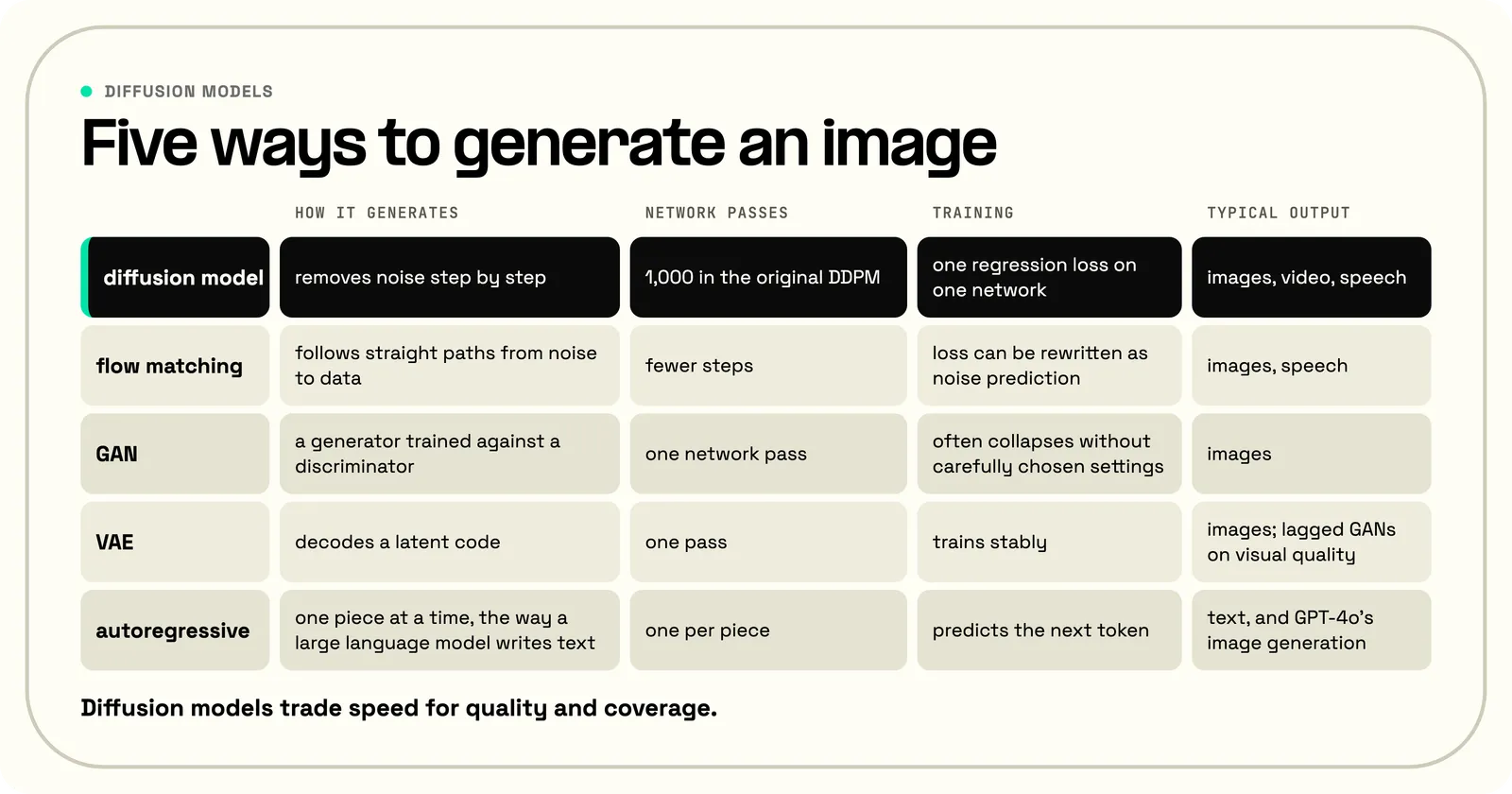
Diffusion models trade speed for quality and coverage. A GAN or a VAE generates in one network pass; a diffusion model needs many passes but matches or beats both on image quality and covers more of the data's variety.

A generative adversarial network, proposed by Goodfellow and colleagues in 2014, trains a generator against a discriminator that tries to tell real samples from generated ones.

A GAN's training often collapses without carefully chosen settings, as Dhariwal and Nichol note.

A variational autoencoder, from Kingma and Welling, learns to compress data into a latent code and decode it back. It trains stably and samples in one pass.

Dhariwal and Nichol note that likelihood-based models such as VAEs have lagged GANs on visual quality.

Flow matching differs from standard diffusion in the path it trains on: straight or nearly straight lines from noise to data, which need fewer steps.

Autoregressive image models generate an image piece by piece, the way a large language model writes text. OpenAI describes GPT-4o's image generation this way.

Diffusion models in speech and voice AI

Diffusion and flow-matching models generate speech by refining a whole stretch of audio over a set number of steps, and on a live call every step adds compute before that audio can play.

A text-to-speech pipeline usually has two stages: an acoustic model turns text into a spectrogram, a time-frequency picture of sound, and a vocoder turns the spectrogram into a waveform.

Diffusion can run at either stage, and a call pays for both. Grad-TTS generates spectrograms with a score-based diffusion model; DiffWave is a diffusion vocoder.

NaturalSpeech 2 uses latent diffusion. Voicebox, Matcha-TTS and F5-TTS use flow matching, which a vendor may also call diffusion-based.

F5-TTS shows the cost of steps. On an RTX 3090 graphics card it took 1.5 seconds to generate 10 seconds of speech with 16 steps and 3.1 seconds with 32. Twice the steps cost twice the compute, so nearly all the time goes into the steps.

Those timings already include classifier-free guidance, which the authors note doubles inference time: the network runs twice at each step, once with the text and once without.

Neither figure is time to first audio. F5-TTS pads the text to the full length of the speech and denoises the whole clip at once, so no audio exists until the last step finishes. The papers cited here do not report time to first audio.

For voice AI agents, step count therefore sits inside the latency budget, on top of speech recognition and the language model. A few-step model can matter more than a slightly better voice.

The test for any text-to-speech model behind a voice agent is time to first audio on real calls, not quality on a clean benchmark clip.

Frequently asked questions

Who invented diffusion models?

Jascha Sohl-Dickstein and colleagues introduced diffusion models in a 2015 paper on non-equilibrium thermodynamics. Yang Song and Stefano Ermon developed the related score-based approach in 2019.

Jonathan Ho, Ajay Jain and Pieter Abbeel set a state-of-the-art image-quality score in 2020, in the paper that named DDPMs.

Is ChatGPT a diffusion model?

ChatGPT is not a diffusion model. Its language models generate text one token at a time, which makes them autoregressive. OpenAI's GPT-4 technical report describes the model as pre-trained to predict the next token in a document.

For images, OpenAI's March 2025 system card states that "Unlike DALL·E, which operates as a diffusion model, 4o image generation is an autoregressive model natively embedded within ChatGPT."

What is the diffusion decision model?

The diffusion decision model, also called the drift-diffusion model, is a psychology model of how people make fast two-choice decisions, not a generative AI model.

The model treats a decision as evidence that builds up noisily until it reaches one of two thresholds, as Ratcliff and McKoon describe. The shared name comes from the shared mathematics of random noise accumulating over time.

Are diffusion models still used?

Diffusion models are still in wide use. Sora (2024) is a diffusion transformer, recent text-to-image research builds on rectified flow, a flow-matching method, and diffusion language models such as LLaDA and Mercury arrived in 2025.

Are video models diffusion models?

Many video generation models are diffusion models. OpenAI describes Sora as a diffusion transformer that denoises patches of video. Ho and colleagues built an early video diffusion model in 2022.

Video can also be generated other ways. The Sora report's survey of earlier work lists recurrent networks, GANs and autoregressive transformers alongside diffusion models.

Sources

• Sohl-Dickstein, J., Weiss, E. A., Maheswaranathan, N., and Ganguli, S. (2015). Deep unsupervised learning using nonequilibrium thermodynamics. ICML 2015.
• Song, Y., and Ermon, S. (2019). Generative modeling by estimating gradients of the data distribution. NeurIPS 2019.
• Ho, J., Jain, A., and Abbeel, P. (2020). Denoising diffusion probabilistic models. NeurIPS 2020.
• Song, Y., Sohl-Dickstein, J., Kingma, D. P., Kumar, A., Ermon, S., and Poole, B. (2021). Score-based generative modeling through stochastic differential equations. ICLR 2021.
• Song, J., Meng, C., and Ermon, S. (2021). Denoising diffusion implicit models. ICLR 2021.
• Dhariwal, P., and Nichol, A. (2021). Diffusion models beat GANs on image synthesis. NeurIPS 2021.
• Ho, J., and Salimans, T. (2022). Classifier-free diffusion guidance. arXiv:2207.12598.
• Rombach, R., Blattmann, A., Lorenz, D., Esser, P., and Ommer, B. (2022). High-resolution image synthesis with latent diffusion models. CVPR 2022.
• CompVis. Stable Diffusion, model release and README.
• Meng, C., et al. (2022). SDEdit: guided image synthesis and editing with stochastic differential equations. ICLR 2022.
• Ramesh, A., Dhariwal, P., Nichol, A., Chu, C., and Chen, M. (2022). Hierarchical text-conditional image generation with CLIP latents. arXiv:2204.06125.
• Saharia, C., et al. (2022). Photorealistic text-to-image diffusion models with deep language understanding. NeurIPS 2022.
• Ronneberger, O., Fischer, P., and Brox, T. (2015). U-Net: convolutional networks for biomedical image segmentation. MICCAI 2015.
• Peebles, W., and Xie, S. (2023). Scalable diffusion models with transformers. ICCV 2023.
• Lipman, Y., Chen, R. T. Q., Ben-Hamu, H., Nickel, M., and Le, M. (2023). Flow matching for generative modeling. ICLR 2023.
• Liu, X., Gong, C., and Liu, Q. (2023). Flow straight and fast: learning to generate and transfer data with rectified flow. ICLR 2023.
• Esser, P., et al. (2024). Scaling rectified flow transformers for high-resolution image synthesis. ICML 2024.
• Song, Y., Dhariwal, P., Chen, M., and Sutskever, I. (2023). Consistency models. ICML 2023.
• Ho, J., Salimans, T., Gritsenko, A., Chan, W., Norouzi, M., and Fleet, D. J. (2022). Video diffusion models. NeurIPS 2022.
• OpenAI (2024). Video generation models as world simulators.
• Kong, Z., Ping, W., Huang, J., Zhao, K., and Catanzaro, B. (2021). DiffWave: a versatile diffusion model for audio synthesis. ICLR 2021.
• Watson, J. L., et al. (2023). De novo design of protein structure and function with RFdiffusion. Nature 620.
• Song, Y., Shen, L., Xing, L., and Ermon, S. (2022). Solving inverse problems in medical imaging with score-based generative models. ICLR 2022.
• Chi, C., et al. (2023). Diffusion Policy: visuomotor policy learning via action diffusion. RSS 2023.
• Carlini, N., et al. (2023). Extracting training data from diffusion models. USENIX Security 2023.
• Goodfellow, I. J., et al. (2014). Generative adversarial networks. NeurIPS 2014.
• Kingma, D. P., and Welling, M. (2014). Auto-encoding variational Bayes. ICLR 2014.
• Nie, S., et al. (2025). Large language diffusion models. NeurIPS 2025.
• Inception Labs, et al. (2025). Mercury: ultra-fast language models based on diffusion. arXiv:2506.17298.
• OpenAI (2023). GPT-4 technical report. arXiv:2303.08774.
• OpenAI (2025). Addendum to GPT-4o system card: 4o image generation.
• Wang, C., et al. (2023). Neural codec language models are zero-shot text to speech synthesizers. arXiv:2301.02111.
• Popov, V., Vovk, I., Gogoryan, V., Sadekova, T., and Kudinov, M. (2021). Grad-TTS: a diffusion probabilistic model for text-to-speech. ICML 2021.
• Shen, K., et al. (2023). NaturalSpeech 2: latent diffusion models are natural and zero-shot speech and singing synthesizers. arXiv:2304.09116.
• Le, M., et al. (2023). Voicebox: text-guided multilingual universal speech generation at scale. NeurIPS 2023.
• Mehta, S., Tu, R., Beskow, J., Székely, É., and Henter, G. E. (2024). Matcha-TTS: a fast TTS architecture with conditional flow matching. ICASSP 2024.
• Chen, Y., et al. (2024). F5-TTS: a fairytaler that fakes fluent and faithful speech with flow matching. arXiv:2410.06885.
• Richter, J., Welker, S., Lemercier, J.-M., Lay, B., and Gerkmann, T. (2023). Speech enhancement and dereverberation with diffusion-based generative models. IEEE/ACM Transactions on Audio, Speech, and Language Processing 31.
• Ratcliff, R., and McKoon, G. (2008). The diffusion decision model: theory and data for two-choice decision tasks. Neural Computation 20(4).
• Telnyx. Deepfake detection. Telnyx developer documentation.