Pooling reduces feature-map size in neural networks. Learn max, average, and global pooling with a simple example and the tradeoffs behind each choice.

Updated August 2026
Pooling is an operation in neural networks that summarizes values from a local region of a feature map. It often reduces the spatial dimensions passed to later layers. PyTorch defines MaxPool2d as a maximum operation over local input planes and documents the resulting output-shape calculation.
This content was generated with the assistance of AI. Our AI prompt chain workflow is carefully grounded and preferences .gov and .edu citations when available. All content is reviewed by a Telnyx employee to ensure accuracy, relevance, and a high standard of quality.
A pooling window moves across a feature map and replaces each local patch with one value. The rule determines the output. Max pooling keeps the largest value in each patch. Average pooling calculates the mean. The window size and stride determine how much the feature map is reduced.
For a 2 by 2 patch with values [1, 3; 2, 4], max pooling outputs 4. Average pooling outputs 2.5. Neither output preserves the exact original layout.
A 2 by 2 pooling window with stride 2 reduces an even-sized feature map's height and width by half when padding and dilation are zero. PyTorch's output-shape formula supports that result.
| Type | Operation | Useful when |
|---|---|---|
| Max pooling | Keeps the largest value in each window | Strong local feature presence matters |
| Average pooling | Calculates the mean of each window | Smooth aggregate response is useful |
| Global average pooling | Averages each full feature map | Converting feature maps into a compact vector |
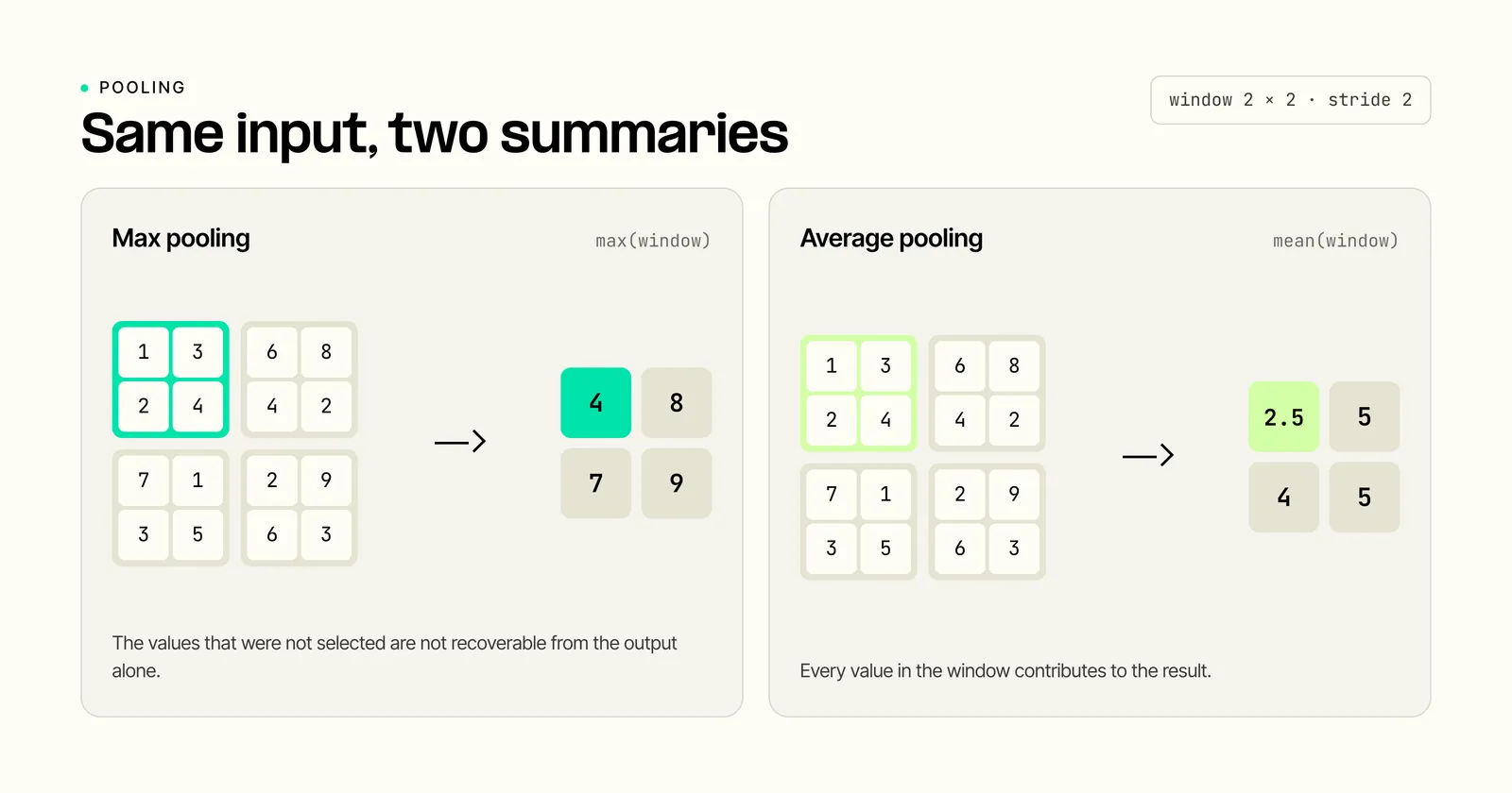
Max pooling selects the largest activation from each local window. PyTorch describes the operation mathematically and exposes an option to return the selected indices, which are needed by MaxUnpool2d for partial inversion. Values that were not selected are not recoverable from the pooled output alone.
Max pooling is common in classic CNN architectures, but it is a design choice rather than a requirement. Its value depends on the task, data, and later layers.
Average pooling replaces each window with its average activation. It keeps a smoother summary than max pooling because every value contributes to the output. It can be useful when the aggregate strength of a feature matters more than a single strong response.
Global average pooling applies averaging across the full spatial dimensions of each feature map. It is often used near a model’s output to reduce each map to one value per channel.
Avoid or limit pooling when fine spatial detail is central to the task. A peer-reviewed small-object segmentation study identifies information loss from convolution and pooling as a specific problem for small and thin objects, then evaluates its proposed mitigation across 8 segmentation networks.
Segmentation and dense-prediction architectures often compensate with skip connections, learned upsampling, or less aggressive downsampling. The right choice depends on which spatial details the output must preserve.
The right choice should be validated experimentally. Compare the full model under the same training setup, not an isolated layer in a vacuum.
Window size defines how many neighboring values are summarized. Stride defines how far the window moves each time. A 2 by 2 window with stride 2 reduces the height and width by about half when padding does not change the output shape.
Overlapping windows use a stride smaller than the window. They retain more local overlap but increase computation and output size. Record both settings when comparing architectures. Saying a model "uses max pooling" without its window and stride leaves out the part that determines the actual downsampling.
Global average pooling averages each complete feature map into one value. If the final convolutional layer has 512 channels, global average pooling turns each channel's height by width map into one number, producing a vector of 512 values. This is a dimensional consequence of the operation, not a benchmark claim.
The Network in Network paper proposed global average pooling as a replacement for fully connected output layers. The authors argued that the design made feature maps easier to interpret and reduced overfitting because the pooling step added no trainable parameters.
The GPU architecture guide gives useful context for why feature-map size affects compute. For architecture selection more broadly, see Telnyx's machine learning framework explainer.
Hold the dataset, training budget, augmentation, and evaluation metric constant. Then compare candidate pooling operations with the same surrounding architecture. Inspect more than the headline accuracy. Look for changes by image size, object size, class, and failure mode.
Pooling can improve one metric while damaging the detail needed for a critical subset of inputs. Visualize activation maps or error examples where possible. That is more useful than declaring one pooling type universally better.
The AI classification guide explains how networks turn learned features into labels. The inference hardware guide connects architecture choices to the systems used to run the resulting model.
The training versus inference guide explains how architecture choices affect two different stages of the model lifecycle.
Image classification provides a named example. Network in Network used global average pooling after its final feature maps and reported 8.81% test error on CIFAR-10 with dropout and data augmentation. That historical result does not isolate pooling as the sole cause, but it documents the operation inside a measured architecture rather than treating it as an abstract layer.
The same segmentation study provides the counterexample: repeated downsampling can erase small and thin structures. The classification and segmentation findings point to different design needs. Compact features can help a classifier, while precise location matters to segmentation.
Start with the feature-map shape before and after every downsampling layer. A model that reduces an image too aggressively can make small or closely spaced objects impossible to recover in later layers.
Use validation examples that stress the detail your application depends on. For instance, compare performance on small objects and boundary-heavy images, not only the aggregate score. The result should decide whether pooling, stride, or an alternative downsampling method is appropriate.
Pooling layers typically have no learned weights, but reducing spatial dimensions can reduce the computation and the size of later layers. The total parameter effect depends on the architecture that follows the pooling layer.
A convolution uses learned filters to transform the input. Standard max and average pooling use a fixed aggregation rule to summarize a local region. Both can change spatial dimensions, but they play different roles in a neural-network architecture.
No. Max pooling emphasizes the strongest activation, while average pooling preserves an aggregate response. The better option depends on the data, objective, architecture, and observed validation results. Test the alternatives rather than relying on a general rule.