What is a probabilistic model? How it works, types, and examples

Updated October 2026

A probabilistic model is a machine learning model that describes data with probability distributions. Instead of returning one answer, it returns the possible outcomes with a probability for each, so its output shows how sure it is. Spam filters, speech recognizers and large language models all work this way.

The same idea runs a spam filter and a chatbot. A large language model predicts a probability for every possible next word, then picks one at random from the likeliest. That is why one question can get two different answers.

What is a probabilistic model?

A probabilistic model treats what it does not know as a random variable and gives each possible value a probability.

In Murphy's terms, a random variable is a quantity whose value is unknown or could change, such as the face of a rolled die. Its possible values form the sample space.

A caller tells a voice AI agent "I want to cancel my order." The caller's intent is the unknown, and its sample space is cancel, billing or other.

Instead of answering only "cancel", a probabilistic intent classifier might return cancel 0.86, billing 0.09 and other 0.05.

The probabilities add up to 1, and their spread shows how sure the model is. A result of cancel 0.45, billing 0.40 and other 0.15 would mean the model is unsure, and that call is one to hand to a person.

Doubt has two sources. Model uncertainty comes from what the model has not yet learned, such as few training calls phrased like this one, and more data reduces it.

Data uncertainty is built into the world. A sentence can genuinely mean two things, just as the next toss of a fair coin cannot be predicted.

An ordinary classifier's probabilities carry only the second kind. It uses one best setting of its parameters, an approach Murphy notes "can suffer from overfitting and overconfidence".

The Bayesian models covered below carry the first kind too.

In statistics, a probability model is the simplest case: a sample space with a probability for each outcome. In machine learning, the probabilities also depend on an input, such as the caller's words.

How probabilistic models work

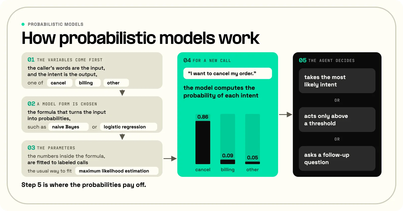
A probabilistic model is built in five steps. For the caller's intent classifier:

1. The variables come first: the caller's words are the input, and the intent is the output, one of cancel, billing or other.
2. A model form is chosen: the formula that turns the input into probabilities, such as naive Bayes or logistic regression, both covered below.
3. The parameters, the numbers inside the formula, are fitted to labeled calls. For naive Bayes, they include how often each word appears in each intent.
4. For a new call, the model computes the probability of each intent: cancel 0.86, billing 0.09, other 0.05.
5. The agent decides: it takes the most likely intent, acts only above a threshold, or asks a follow-up question.

The usual way to fit step 3 is maximum likelihood estimation. In Murphy's words, it picks "the parameters that assign the highest probability to the training data".

If 60 of 100 cancellation calls contain "cancel", the estimate is 0.6, because that value makes the labeled calls most likely.

Step 5 is where the probabilities pay off. A classifier in production returns a probability, and the application applies its own threshold to turn it into an action.

Types of probabilistic models

Probabilistic models are sorted three ways, and the groups overlap: by what they model, by how they draw dependencies, and by whether they use hidden variables.

Generative and discriminative models

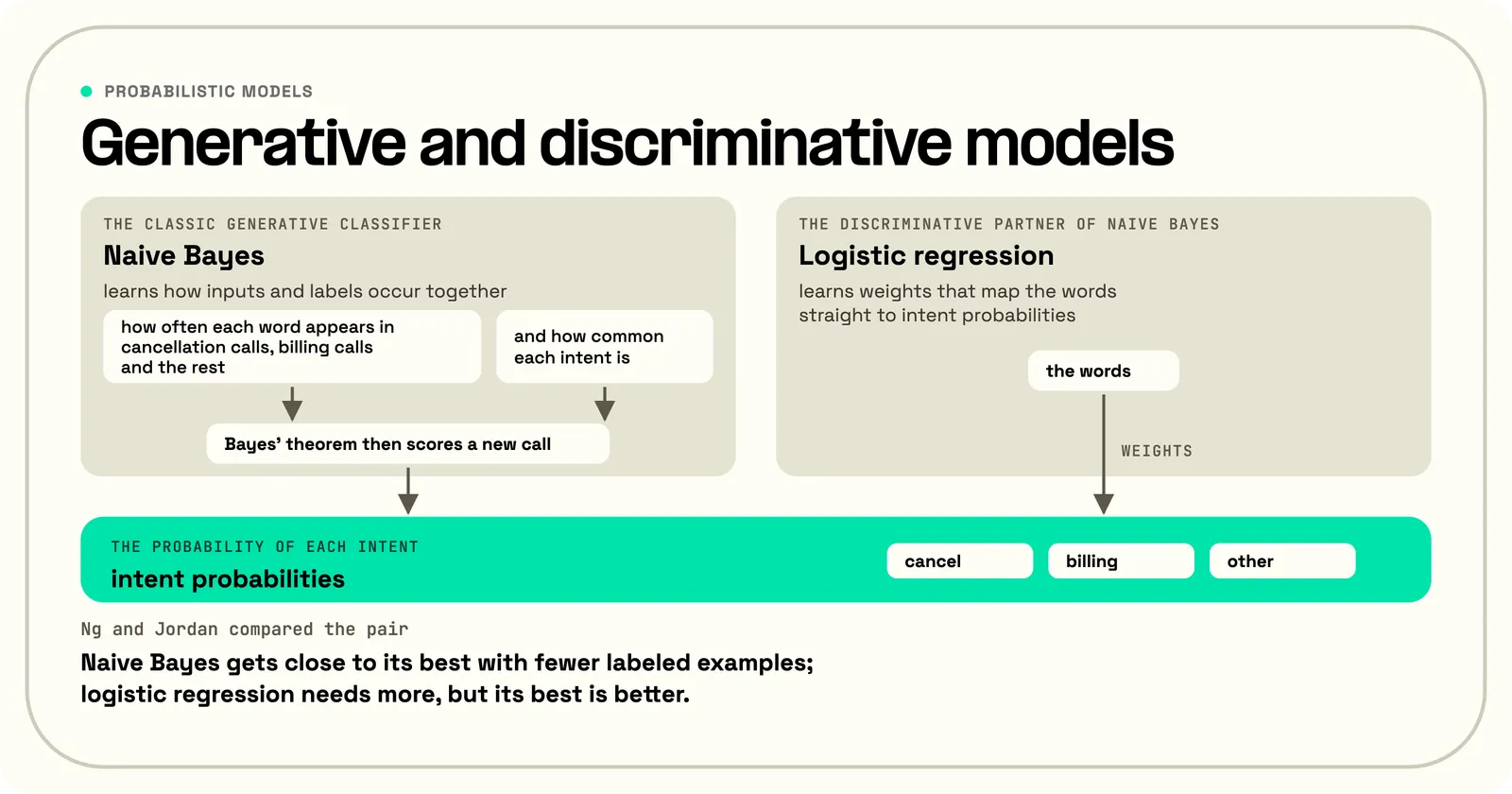
A generative model learns how inputs and labels occur together. A discriminative model learns only the label given the input.

So a generative classifier "can be used to generate examples" of each class, in Murphy's words, while a discriminative one "can only be used to discriminate between different classes".

A generative model of calls could produce made-up examples of each intent. Logistic regression, a discriminative model, can only tell the intents apart.

Naive Bayes is the classic generative classifier. For the caller, it learns how often each word appears in cancellation calls, billing calls and the rest, and how common each intent is. Bayes' theorem then scores a new call.

It is "naive" because it treats each word as independent evidence once the intent is known, which real words are not.

Fitting naive Bayes takes little more than counting. It also copes with missing inputs: if the transcript loses part of the call, it can still score the words it has.

A discriminative model has "no principled solution" to missing inputs, Murphy notes, because it assumes every input is there.

Logistic regression is the discriminative partner of naive Bayes. It learns weights that map the words straight to intent probabilities.

Ng and Jordan compared the pair. Naive Bayes gets close to its best with fewer labeled examples; logistic regression needs more, but its best is better.

Other generative models include Gaussian mixture models, hidden Markov models and diffusion models, which generate images.

Probabilistic graphical models

A probabilistic graphical model draws the dependencies between variables as a graph. Each node is a random variable, and each edge is a direct dependency. A missing edge means no direct dependency.

Naive Bayes is a small one: an intent node with an arrow to every word. The missing edges between the words are its naive assumption.

Murphy's larger example links four variables: whether the season is cloudy, whether the sprinkler is on, whether it rains, and whether the grass is wet. Clouds affect the sprinkler and the rain, and both of those affect the grass.

A graph with directed edges and no cycles, where following the arrows never leads back to the start, is called a Bayesian network.

Murphy notes "there is nothing inherently Bayesian about such models": the name does not mean the Bayesian approach covered below.

Using the graph to answer a question, such as how likely rain is given wet grass, is called inference. That is a different sense of the word from running a trained model in production.

When the edges are read as causes, as in the sprinkler example, a graphical model becomes a tool for causal inference. Murphy cautions that a statistical dependence on its own does not show a cause.

Latent variable models

A latent variable model explains data through causes it never observes.

A Gaussian mixture model assumes each data point came from one of several hidden clusters, each a bell-shaped Gaussian distribution. If call lengths bunch around two minutes and around twelve, a mixture of two clusters can describe them.

The expectation-maximization (EM) algorithm fits it in two alternating steps. It estimates how likely each point is to belong to each cluster, refits each cluster to all the points weighted by those probabilities, and repeats.

Latent Dirichlet allocation does the same for text. Each document is a mix of hidden topics, and each topic favors certain words.

A hidden Markov model handles sequences. Its hidden states, such as the speech sounds behind a stretch of audio, follow each other with transition probabilities.

Each state also has emission probabilities for what it produces. The Viterbi algorithm then finds the most likely sequence of hidden states behind what was observed.

For decades, most speech recognizers used hidden Markov models inside the acoustic model to track how speech sounds unfold over time. The hybrid systems that brought in deep neural networks in the 2010s kept them.

Bayesian inference in probabilistic models

Bayesian inference updates a probability when evidence arrives, using Bayes' theorem:

posterior = likelihood × prior ÷ evidence

Suppose 1 in 10 calls is a cancellation, the prior. The word "cancel" appears in 60% of cancellation calls and 2% of other calls, the likelihoods. For a call that says "cancel":

• 0.1 × 0.6 = 0.06 for cancellations, prior times likelihood
• 0.9 × 0.02 = 0.018 for the other calls
• 0.06 + 0.018 = 0.078, the evidence
• 0.06 ÷ 0.078 = about 0.77, the posterior, up from 0.1

Bayesian models apply the same rule to their own parameters. Maximum likelihood says 60% of cancellation calls contain "cancel" and stops there.

A Bayesian model treats that rate as unknown too: probably near 60%, possibly 50% or 70%. It averages its predictions over that range, which is wide after ten labeled calls and narrow after ten thousand.

For most models, the evidence term means adding up over every possible setting of the parameters, which is impractical. Markov chain Monte Carlo approximates the posterior by drawing samples from it.

Variational inference fits a simpler distribution in the posterior's place. Priors, posteriors and the trade-offs of the approach are covered in Bayesian machine learning.

Applications of probabilistic models

Probabilistic models run wherever an answer comes with doubt. Ghahramani lists scientific data analysis, machine learning, robotics, cognitive science and artificial intelligence as fields where the framework has "a central role".

• Spam filters, intent detection and sentiment analysis return a probability for each class.
• Image classifiers return a probability for each label.
• Speech recognizers long used hidden Markov models to line speech sounds up with the audio.
• Topic models such as latent Dirichlet allocation find the themes running through a large collection of documents.
• Generative models produce new data: diffusion models create images, and language models write text one token at a time.

Probabilistic models in large language models

A large language model is a probabilistic model of text. Jurafsky and Martin define a language model as one that "assigns a probability to each possible next word". It runs through the same five steps as the intent classifier:

1. The input is the text so far, and the output is the next token, a word or a piece of one.
2. The model form is a large neural network.
3. The parameters are fitted to a large body of text by maximum likelihood, which rewards the network for giving a high probability to the token that actually came next.
4. For a prompt, the model computes a probability for every token in its vocabulary.
5. The application chooses a token, adds it to the text, and repeats.

Bengio and colleagues trained a neural network this way in 2003, fitting it to "maximize the log-likelihood of the training data".

Step 5 is where language models differ from the intent classifier. Always taking the most likely token sounds safe, but Holtzman and colleagues found that it produces text that is "bland, incoherent, or gets stuck in repetitive loops".

So most systems sample from the distribution, shaped by two controls. Suppose the model rates the word after "cancel my" as order 0.5, subscription 0.3 and account 0.2.

Temperature rescales those probabilities. At 0.5 they sharpen to about 0.66, 0.24 and 0.11; at 2 they flatten to about 0.42, 0.32 and 0.26. Values below 1 tilt the choice toward likely tokens.

Top-p sampling, also called nucleus sampling, keeps only the smallest set of tokens whose probabilities add up to p. With top-p at 0.8, only "order" and "subscription" stay in the running.

Outputs can vary even at temperature 0, where the model always takes the most likely token.

He and colleagues traced this to servers processing requests in batches, which changes the arithmetic. In their test, 1,000 runs of one prompt at temperature 0 produced 80 different completions.

How the model's raw scores, its logits, become those probabilities is covered separately.

Advantages and limitations of probabilistic models

Probabilistic models earn their extra work when doubt matters.

Their strengths:

• They report uncertainty an application can act on.
• Their assumptions are explicit, such as the edges in a graphical model, so they can be inspected.

Their limits mostly concern how far those probabilities can be trusted.

Wrong assumptions give wrong probabilities. Naive Bayes counts "cancel" and "cancellation" in one call as separate evidence, so its probabilities overshoot.

Murphy notes the result can be "very extreme posterior class probabilities (very near 0 or 1)".

Probabilities can also be badly calibrated. A model is calibrated when its confidence matches its accuracy: of 100 predictions made at 0.8, about 80 should be right.

Guo and colleagues found that "modern neural networks, unlike those from a decade ago, are poorly calibrated". Their fix, temperature scaling, divides the raw scores by one number chosen on held-out data.

Temperature scaling uses the same math as sampling temperature, but to correct confidence rather than to add randomness.

Small data misleads. A word never seen with an intent gets probability zero under maximum likelihood, the zero-count problem. Smoothing, such as adding one to every count, avoids it.

Exact inference, in the graph and Bayesian senses above, can be expensive, which is why the approximations exist.

What a model's probability does and does not tell an application is covered in logits and confidence.

Probabilistic vs deterministic models

A deterministic model gives the same single answer every time it sees the same input. A probabilistic model gives a distribution over answers.

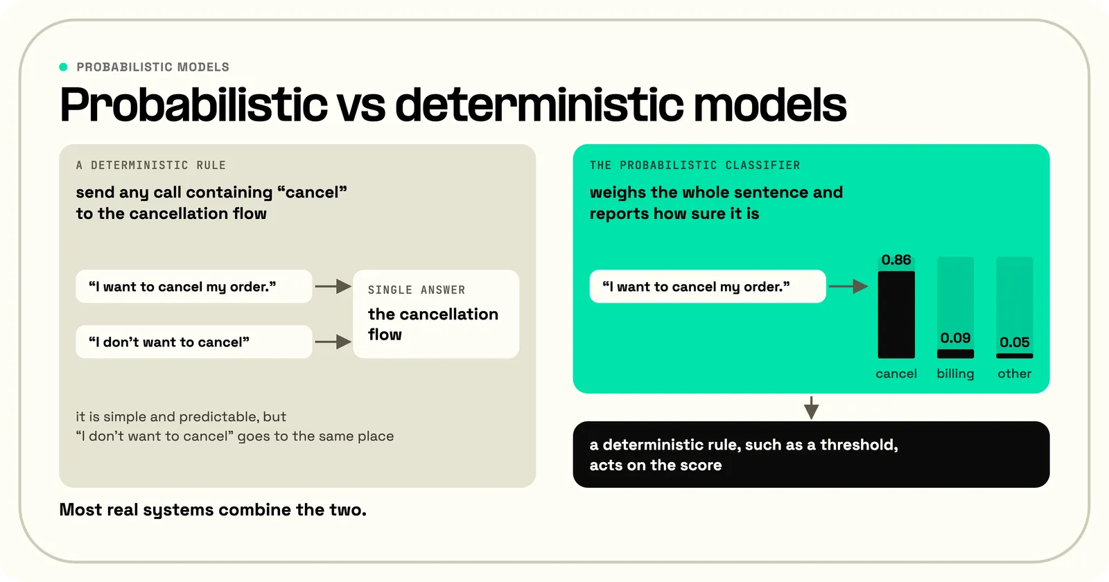
For the caller, a deterministic rule might send any call containing "cancel" to the cancellation flow. It is simple and predictable, but "I don't want to cancel" goes to the same place.

The probabilistic classifier weighs the whole sentence and reports how sure it is.

Deterministic models suit fixed logic, such as calculating a bill or checking a policy. Probabilistic models suit ambiguous input, such as speech, text and images.

Most real systems combine the two. A probabilistic model scores the options, and a deterministic rule, such as a threshold, acts on the score.

"Stochastic" is a near-synonym for probabilistic here, so "deterministic vs stochastic" names the same contrast.

Probabilistic models in voice AI agents

A voice AI agent chains probabilistic models, among them a transcriber, an end-of-turn detector and a language model. Each hands the next a probability rather than a certainty.

The transcriber hears "I want to cancel my order". The Telnyx Speech-to-Text API returns each final transcript with a confidence score from 0.0 to 1.0, such as 0.98.

Partial transcripts report 0.0, because confidence "is only meaningful on final results". An agent can use the score, for example by confirming a low-confidence order number before acting on it.

The end-of-turn detector decides whether the caller has finished. On one of the speech models, end-of-turn detection fires once its confidence that the caller is done passes a threshold.

That threshold is 0.7 by default on the streaming API and 0.8 in AI Assistants. A higher value means fewer premature end-of-turn calls but slightly more latency.

An optional lower threshold can start a speculative reply early.

Then the language model samples a reply. The chat completions API exposes temperature and top-p. Temperature defaults to 0.1, and lower values make the output more deterministic.

The same API can return log probabilities for each output token, and a seed makes sampling repeatable on a best-effort basis.

Teams that build their own pipeline on the Voice API can bridge call audio into the same streaming endpoint and set these thresholds themselves.

Frequently asked questions

What is an example of a probabilistic model?

A naive Bayes spam filter is a classic example. It learns how often words appear in spam and in normal email, then returns the probability that a new message is spam.

Weather forecasts, speech recognizers and large language models are probabilistic too.

Why are LLMs not deterministic?

Because they sample. A large language model computes a probability for every possible next token, then picks one at random from the likeliest, shaped by temperature and top-p.

A low temperature or a fixed seed makes answers far more repeatable, though not always identical.

Is AI probabilistic or deterministic?

Most modern AI models are probabilistic: classifiers return class probabilities, and language models return next-token probabilities. The systems around them are often deterministic, applying fixed rules and thresholds.

Are probabilistic graphical models still used?

Yes, often inside newer models. Ho, Jain and Abbeel define a diffusion model as "a parameterized Markov chain trained using variational inference", and draw it as a directed graphical model.

What is a probability model in statistics?

A probability model lists the possible outcomes, called the sample space, with a probability for each. A fair die is the simplest example: six outcomes, each with probability 1/6.

Machine learning models extend the idea by letting the probabilities depend on an input.

Sources

• Jurafsky, D., and Martin, J. H. (2026). Speech and Language Processing, chapters 3, "N-gram Language Models", and 4, "Logistic Regression and Text Classification", and appendix A, "Hidden Markov Models" (draft of August 19, 2026).
• Murphy, K. P. (2022). Probabilistic Machine Learning: An Introduction. MIT Press.
• Ghahramani, Z. (2015). Probabilistic machine learning and artificial intelligence. Nature, 521.
• Ng, A. Y., and Jordan, M. I. (2002). On discriminative vs. generative classifiers: a comparison of logistic regression and naive Bayes. Advances in Neural Information Processing Systems 14.
• Blei, D. M., Ng, A. Y., and Jordan, M. I. (2003). Latent Dirichlet allocation. Journal of Machine Learning Research, 3.
• Bengio, Y., Ducharme, R., Vincent, P., and Jauvin, C. (2003). A neural probabilistic language model. Journal of Machine Learning Research, 3.
• Holtzman, A., Buys, J., Du, L., Forbes, M., and Choi, Y. (2020). The curious case of neural text degeneration. ICLR 2020.
• Guo, C., Pleiss, G., Sun, Y., and Weinberger, K. Q. (2017). On calibration of modern neural networks. ICML 2017.
• Ho, J., Jain, A., and Abbeel, P. (2020). Denoising diffusion probabilistic models. NeurIPS 2020.
• He, H., and Thinking Machines Lab (2025). Defeating nondeterminism in LLM inference. Thinking Machines Lab: Connectionism.
• Telnyx. Speech-to-Text WebSocket messages, Interim results, End-of-turn detection, AI Assistants transcription settings and Create a chat completion. Telnyx developer documentation.